13. Logistic regression basics⚓︎

Module items⚓︎

R Script file⚓︎

Copy the code below ➜ Paste into [[RStudio console]] ➜ Hit Enter

source(url("https://raw.githubusercontent.com/ttezcann/ssric-reg/refs/heads/main/regression/docs/assets/r-scripts/0_packages_data.R")); 
download.file("https://raw.githubusercontent.com/ttezcann/ssric-reg/refs/heads/main/regression/docs/assets/r-scripts/13-logistic.R", "13-logistic.R"); 
file.edit("13-logistic.R")

Lab assignment⚓︎

Logistic regression

Sample lab assignment⚓︎

Sample: Logistic regression

Learning outcomes⚓︎

1. Define logistic regression analysis
2. Identify situations in which logistic regression is appropriate
3. Interpret Odd Ratios (OR), standardized betas (Std.Beta), and R-squared Tjur value

Suggested reading⚓︎

Logistic regression structure⚓︎

• [[Logistic regression]] is a regression model where;
  • The [[outcome variable]] is
    • A [[dummy variable]], and thus [[binary]], which can take only two values, "1" and "0", such as,
      • pass (1) / fail (0),
      • win (1) / lose (0),
      • alive (1) / dead (0),
      • healthy (1) / sick (0),
      • return (1) / stay (0),
      • voted (1) / didn’t vote (0).
    • Categorical factor variables should also be dummy variable.

• We are interested in showing how factor variables increase or decrease the odds of the outcome variable happening.

  • For example, we may want to see how hours of studying (continuous factor variable; min: 0, max: 7) increases the odds of passing the exam (dummy outcome variable; 1: passing; 0: failing).

    flowchart LR
    subgraph F["Continuous variable"]
        A[Hours of studying<br><br>min: 0, max: 7]
    end
    
    subgraph O["Dummy outcome variable"]
        B[Passing the exam <br><br> 1: passing; 0: failing]
    end
    
    A ==>|May affect| B

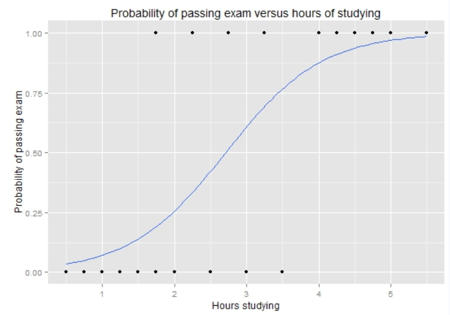
• The figure below shows that the odds of passing the exam increases as the number of study hours increases.

  • For example, students who study very little have a low odds of passing.
  • If a student studies around 2 hours, the odds of passing is still relatively low, around 25%.
  • Around 3 hours of studying, the odds gets close to 50%.
  • If a student studies around 4 hours, the odds of passing becomes much higher, close to 85–90%.
  • If a student studies around 5 or 6 hours, the odds becomes very close to 100%.

  • This means that studying more hours is associated with a higher odds of passing the exam.

    

Logistic regression specifics⚓︎

• [[Logistic regression]] table provides:
  • [[Odds ratio]]: The effect of each factor on the odds of the outcome variable happening. For example, every 1 additional hour of studying increases the odds of passing the exam by about 4.2 times.
    • Odds ratios are interpreted differently from linear regression coefficients.
      • An odds ratio greater than 1 means the factor variable increases the odds of the outcome (OR > 1 is positive).
      • An odds ratio less than 1 means the factor decreases the odds of the outcome (OR < 1 is negative).
    • [[Standard error]]: The margin of uncertainty around each odds ratio. Smaller standard errors mean more precise estimates. Standard errors are right under the odds ratios in parentheses.
  • [[Standardized odds ratio]]: The odds ratio rescaled to allow comparison across factors regardless of their units.
    • This is useful because different variables are measured differently.
      • Age is measured in years.
      • Education is measured in years.
      • Income may be measured in dollars.
      • Occupational prestige may be measured with a score.
    • Standardized odds ratios help us compare which factor has a stronger relative contribution.
  • [[p-value]]: The probability that the observed coefficient is due to chance. A p-value less than 0.05 is considered statistically significant.
  • [[Tjur R-square]]: The Tjur R-square value shows whether adding additional factor variables improve the explanatory power of regression model or not. The adjusted R-squared should be reported as a percentage.

Example: Passing the exam⚓︎

• Here's what a logistic regression table looks like:

  Passing the exam

  Factors	Odds Ratios	std. OR	p
  (Intercept)	0.03 (0.01)	0.90 (0.03)	0.001*
  Drinking coffee before exam	1.08 (0.12)	1.03 (0.04)	0.430
  Hours of studying	4.20 (0.35)	2.40 (0.12)	0.001*
  Having a full-time job	0.45 (0.08)	0.70 (0.05)	0.001*
  Observations	500
  R² Tjur	0.312

  Which factors are significant and which one is nonsignificant?

  • Hours of studying and Having a full-time job are significant (p < 0.05, ***)
  • Drinking coffee before exam is nonsignificant; it has no effect on passing the exam (p > 0.05)

  Which factor is positive and which one is negative?

  • Hours of studying is positive (p < 0.05 and OR > 1; 4.20)
  • Having a full-time job is negative (p < 0.05 and OR < 1; 0.45)

• How to interpret positive odd ratio (OR)?

  • An hour increase in studying increases the odds of passing the exam by 4.20 times.
• How to interpret negative odd ratio (OR)?
  • Having a full-time job decreases the odds of passing the exam by 2.22 times compared to not having a full-time job.
    • We see 0.45 odd ratio on the table.
      • When reporting negative odd ratios, we divide 1 by the negative odd ratios and standardized odd ratios.
        • Type “calculator” on Google
        • Divide 1 by the odd ratios and standardized odd ratios
          • 1 / 0.45 = 2.22
          • 1 / 0.70 = 1.43

  • If we included "Not having a full-time job" to the model, instead of `Having a full-time job", we'd have this table:

    Passing the exam

    Factors	Odds Ratios	std. OR	p
    (Intercept)	0.03 (0.01)	0.90 (0.03)	0.001*
    Drinking coffee before exam	1.08 (0.12)	1.03 (0.04)	0.430
    Hours of studying	4.20 (0.35)	2.40 (0.12)	0.001*
    Not having a full-time job	2.22 (0.08)	1.43 (0.05)	0.001*
    Observations	500
    R² Tjur	0.312

GSS example: Predicting perceiving as higher class⚓︎

• Logistic regression analysis will answer the following question:
  • Do factor variables significantly determine the odds of being a higher class? In other words, do they significantly increase or decrease the odds of being a higher class?
    • If so, what is the contribution of each factor variable on the odds of being a higher class?
    • If so, what is the strength of each factor variable’s contribution on the odds of being a higher class?

Find the variables in Variables in GSS page⚓︎

• In this analysis, we propose a cause-and-effect relationship in which these factor variables may affect (increase or decrease) the odds of being a higher class.

  flowchart LR
  subgraph C0[Continuous factor variable]
      direction TB
      A[Education]
  end
  
  subgraph D0[Dummy factor variables]
      subgraph I0[Sex]
          direction TB
          I1[Being male]
          I2[Being female]
      end
  
      subgraph M0[Race]
          direction TB
          M1[Being white]
          M2[Being nonwhite]
  
      end
  end
  
  subgraph O0[Dummy outcome variable]
      E[Class<br><br>1: Perceiving as higher class <br><br> 0: Perceiving as lower class]
  end
  
  A -.->|May affect| E
  I0 -.->|May affect| E
  M0 -.->|May affect| E

• We want to make sure that educ is a continuous variable or usable ordinal variables (Ordinal ✅), and need to see the values of categorical variables for dummy variable codes (both outcome and factor variables).

• First, let's create the dummy variables first.
  • We'll create dummy variables for:
    • The outcome variable, class, and
    • The factor variables: sex and race.

[[Dummy variable]]: Categorical (nominal/ordinal) #code⚓︎

• We'll merge "1: Lower class" and "2: Working class", and call it lowerclass;
• We'll merge "3: Middle class" and "4: Upper class" and call it higherclass.
• We'll include higherclass in the model, and lowerclass will be our omitted comparison category.

• Model code

  1 2 3 4 5 6 7

  gss$dummyvar1 <- ifelse(gss$orig_var == value, 1, 0 | gss$orig_var == value, 1, 0, label = "Dummy variable's variable label") gss$dummyvar2 <- ifelse(gss$orig_var == value, 1, 0 | gss$orig_var == value, 1, 0, label = "Dummy variable's variable label")

• Working code

  1 2 3 4 5 6 7

  gss$lowerclass <- ifelse(gss$class == 1, 1, 0 | gss$class == 2, 1, 0, label = "Perceiving as lower class") gss$higherclass <- ifelse(gss$class == 3, 1, 0 | gss$class == 4, 1, 0, label = "Perceiving as higher class")

  Code explanation: Click to expand

  • Line 1: We put the new variable name here:
    • lowerclass here ➜ dummyvar1
      • It's better to write something simple and memorable, thus lowerclass.
  • Line 2: We put the original variable that we want to create a dummy variable.
    • class here ➜ orig_var
    • Since we want to merge 1 "Lower class" and 2 "Working class", we put gss$class == 1, 1, 0 | gss$class == 2, 1, 0 here ➜ gss$orig_var == value, 1, 0 | gss$orig_var == value, 1, 0
      • The whole code with the last 1, 0 means:
        • "if class is 1 or 2, create a new variable called lowerclass, assign them “1”, and assign the rest “0”".
  • Line 3: We write this new dummy variable's variable label here "Perceiving as lower class"
  • Line 5: We put the new variable name here:
    • higherclass here ➜ dummyvar1
      • It's better to write something simple and memorable, thus higherclass.
  • Line 6: We put the original variable that we want to create a dummy variable.
    • class here ➜ orig_var
    • Since we want to merge 3 "Middle class" and 4 "Upper class", we put gss$class == 3, 1, 0 | gss$class == 4, 1, 0 here ➜ gss$orig_var == value, 1, 0 | gss$orig_var == value, 1, 0
      • The whole code with the last 1, 0 means:
        • "if class is 3 or 4, create a new variable called higherclass, assign them “1”, and assign the rest “0”".
  • Line 7: We write this new dummy variable's variable label here "Perceiving as higher class"
  • Creating a dummy variable is in a way recoding a variable, and thus creating a new variable.
  • Running these codes will create two more variables in GSS dataset, lowerclass, and higher.
    • That's it, two more variables, do not expect to see an output.

[[Dummy variable]]: Categorical (binary) #code⚓︎

• We'll create a dummy variable for male;
• We'll create a dummy variable for female;
• We'll include female in the model, and male will be our omitted comparison category.

• Model code

  1 2 3 4 5 6 7

  gss$dummyvar1 <- ifelse(gss$orig_var == value, 1, 0, label = "Dummy variable's variable label") gss$dummyvar2 <- ifelse(gss$orig_var == value, 1, 0, label = "Dummy variable's variable label")

• Working code

  1 2 3 4 5 6 7

  gss$male <- ifelse(gss$sex == 1, 1, 0, label = "Being male") gss$female <- ifelse(gss$sex == 2, 1, 0, label = "Being female")

  Code explanation: Click to expand

  • Line 1: We put the new variable name here:
    • male here ➜ dummyvar1
      • It's better to write something simple and memorable value label here, thus male.
  • Line 2: We put the original variable that we want to create a dummy variable.
    • sex here ➜ orig_var
    • since 1 is "male" in GSS dataset, we put 1 here ➜ value
      • The whole code with the last 1, 0 means:
        • "if sex is 1, create a new variable called male, assign them “1”, and assign the rest “0”".
  • Line 3: We write this new dummy variable's variable label here "Being male"
  • Line 5: We put the new variable name here:
    • female here ➜ dummyvar2
      • It's better to write something simple and memorable here, thus female.
  • Line 6: We put the original variable that we want to create a dummy variable.
    • sex here ➜ orig_var
    • since 2 is "female" in GSS dataset, we put 2 here ➜ value
      • The whole code with the last 1, 0 means:
        • "if sex is 2, create a new variable called female, assign them “1”, and assign the rest “0”".
  • Line 7: We write this new dummy variable's variable label here "Being female"
  • Creating a dummy variable is in a way recoding a variable, and thus creating a new variable.
  • Running these codes will create two more variables in GSS dataset, male and female.
    • That's it, two more variables, do not expect to see an output.

[[Dummy variable]]: Categorical (nominal/ordinal) #code⚓︎

• We'll keep "1: White" and call it white;
• We'll merge "2: Black" and "3: Other" and call it nonwhite.
• We'll include nonwhite in the model, and white will be our omitted comparison category.

• Model code

  1 2 3 4 5 6 7

  gss$dummyvar1 <- ifelse(gss$orig_var == value, 1, 0, label = "Dummy variable's variable label") gss$dummyvar2 <- ifelse(gss$orig_var == value | gss$orig_var == value, 1, 0, label = "Dummy variable's variable label")

• Working code

  1 2 3 4 5 6 7

  gss$white <- ifelse(gss$race == 1, 1, 0, label = "Being white") gss$nonwhite <- ifelse(gss$race == 2 | gss$race == 3, 1, 0, label = "Being nonwhite")

  Code explanation: Click to expand

  • Line 1: We put the new variable name here:
    • white here ➜ dummyvar1
      • It's better to write something simple and memorable, thus white.
  • Line 2: We put the original variable that we want to create a dummy variable.
    • race here ➜ orig_var
    • since 1 is "white" in GSS dataset, we put 1 here ➜ value
      • The whole code with the last 1, 0 means:
        • "if race is 1, create a new variable called white, assign them “1”, and assign the rest “0”".
  • Line 3: We write this new dummy variable's variable label here "Being white"
  • Line 5: We put the new variable name here:
    • nonwhite here ➜ dummyvar1
      • It's better to write something simple and memorable, thus nonwhite.
  • Line 6: We put the original variable that we want to create a dummy variable.
    • race here ➜ orig_var
    • Since we want to merge 2 "Black" and 3 "Other", we put gss$race == 2 | gss$class == 3, 1, 0 here ➜ gss$orig_var == value | gss$orig_var == value, 1, 0
      • The whole code with the last 1, 0 means:
        • "if race is 2 or 3, create a new variable called nonwhite, assign them “1”, and assign the rest “0”".
  • Line 7: We write this new dummy variable's variable label here "Being nonwhite"
  • Creating a dummy variable is in a way recoding a variable, and thus creating a new variable.
  • Running these codes will create two more variables in GSS dataset, white, and nonwhite.
    • That's it, two more variables, do not expect to see an output.

[[Logistic regression]] #code⚓︎

• Model code

  1 2	model1 <- glm(dummy_outcome_here ~ factor1_here + factor2_here + factor3_here, data = gss, family = binomial(link="logit")) tab_model(model1, show.std = T, show.ci = F, collapse.se = T)

• Working code

  1 2	model1 <- glm(higherclass ~ educ + female + nonwhite, data = gss, family = binomial(link="logit")) tab_model(model1, show.std = T, show.ci = F, collapse.se = T)

  Code explanation

  • Line 1: We put higherclass here ➜ outcome_here; educ here ➜ factor1_here; female here ➜ factor2_here; nonwhite here ➜ factor3_here.
    • Outcome variable variable first; then, factor variables separated by plus (+).
  • Line 2: Check the first argument: model1. If this is model1, then we should use model1 here
    • This needs to be model1, otherwise this code won't work.

[[Logistic regression]] #output⚓︎

Perceiving as higher class

[[Logistic regression]] with dummy variables #interpretation⚓︎