08. Probabilistic sampling

Module items¶

R Script file code¶

• [[Copy the code]] below ➜ Paste into [[RStudio console]] ➜ Hit Enter.

  • source(url("https://raw.githubusercontent.com/ttezcann/ssric-reg/refs/heads/main/docs/assets/r-scripts/0-packages-data.R")); 
    (function(f="08-sampling.R"){if(!file.exists(f)){download.file("https://raw.githubusercontent.com/ttezcann/ssric-reg/refs/heads/main/docs/assets/r-scripts/08-sampling.R",f,mode="wb");file.edit(f)}else{download.file("https://raw.githubusercontent.com/ttezcann/ssric-reg/refs/heads/main/docs/assets/r-scripts/08-sampling.R",gsub(".R","-original.R",f),mode="wb");file.edit(gsub(".R","-original.R",f))}})()
    

    • When this R script file opens in a new tab, [[Save R script file|save your previous R script file(s)]], and
      • Close the previous tabs (R Script files), which you can find later in the [[Files tab]].

Lab assignment¶

Sampling

Sample lab assignment¶

Sample: Sampling

Suggested reading¶

Learning outcomes¶

1. Define the concepts of population, sampling frame, and sample in research
2. Differentiate between probability and non-probability sampling methods.
3. Compare and contrast different probability sampling methods
4. Learn how to choose and create dataset using
   1. Non-random sample
   2. Simple random sample
   3. Systematic random sample
5. Evaluate a sampling method's representativeness by comparing the sample mean to the population mean against a threshold
6. Identify advantages and disadvantages of different sampling methods

[[Sampling concepts]]¶

• Is the soup salty?

  • You’ve made soup, and you want to know if it’s salty. What would you do?

  • 

    • Show the answer

      • Stir the soup ➜ This ensures everything is mixed evenly.
      • Take a spoonful ➜ This small portion represents the whole pot.
      • Taste the spoonful ➜ You draw a conclusion about the entire soup.
      • So then,
        • The soup ➜ the population (everyone or everything you want to study).
        • Stirring ➜ ensuring representativeness (making sure the population is not biased or unevenly distributed).
        • The spoonful ➜ the sample (a smaller subset of the population).
        • Tasting ➜ analyzing data (using the sample to make conclusions).

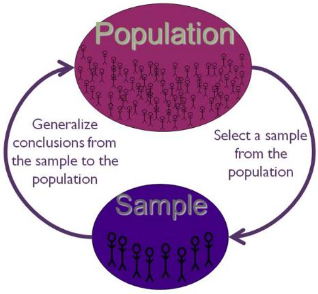
• [[Population]]: The universe of units from which the sample is to be selected.

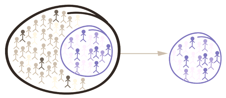
• [[Sample]]: The segment of population that is selected for investigation.
• [[Sampling]]: The process of selecting units from a population so that we can generalize our results over the sample.
• [[Randomness]]: Everyone in the population has an equal chance of being selected
  • 

The mission¶

• We will generate four samples and choose one variable.
  • Our variable is family income, coninc.
    • If the mean family income difference between population (GSS data) and samples diverge a lot, if the mean difference is more than $3,000 (the threshold)**, we can say that sampling method does not represent the population.

• [[Search]] the variable name, conrinc, in Variables in GSS page.

  • Variable name	Variable label	Variable type	Question wording and response categories
    conrinc	Respondents' personal income	Continuous	What is your income in dollars? (Min: $281.5; Max, $123,761.9)

    • First, let's create a descriptive table of family income, coninc.

[[Descriptive table]] #code¶

• [[Model code]]

  • 1	descr(gss$variable_here, out = "v", show = "short")

• [[Working code]]

  • 1	descr(gss$coninc, out = "v", show = "short")

    • Line 1: We put coninc here ➜ variable_here.
      • [[Find this working code in the R script file]].
        • [[Highlighting and running]] this code will generate the output below (which will appear in the [[viewer tab]] of RStudio).

[[Descriptive table]] #output¶

• Basic descriptive statistics

  • variable	variable label	n	NA.prc	mean	sd
    coninc	Respondents' family income	3563	10.61	47738.65	47738.65

[[Descriptive table]] #interpretation¶

• Descriptive table interpretation sample

  The respondents' family income variable shows that the average family income of the respondents is $47,738, with standard deviation $41,328.

• Descriptive table interpretation template

  The [[variable label]] variable shows the average variable label of the respondents is mean, with standard deviation sd.

• Interpretation explanation

  • After the variable label, we add the word of "variable" in your interpretation:
    • "The respondents' education in years variable shows that..."
  • Depending on the variable, we need to tweak some parts of the interpretation.
    • For example, "the average years of education is...", "the average weeks of working is..." etc.
  • We use the mean (mean column) and standard deviation (sd column) in our interpretation.

The range¶

• So then, if the different samples fall in 50,738 - 44,738 dollars range, we'll assume our sampling methods work.

  • flowchart LR
    A["$44,738"] --- B["$47,738"] --- C["$50,738"]
    
    style A fill:stroke:#333,stroke-width:1px
    style B fill:stroke:#333,stroke-width:5px
    style C fill:stroke:#333,stroke-width:1px

• These are the sampling methods we'll use:

  • flowchart TD
        A("GSS data<br/>3,986 respondents")
    
        B("40% <br/>Non-random sampling<br/>1,594 respondents")
        C("30% <br/>Simple random sampling<br/>1,196 respondents")
        D("20% <br/>Systematic random sampling<br/>798 respondents")
    
        A --> B
        A --> C
        A --> D

[[Sampling methods]]¶

• The main distinction between sampling methods is the random selection of participants.
  • In [[non-probability sampling]], a sampling frame is not often available, and participants are not selected randomly.
    • This is called [[non-random sampling]].
  • In [[probability sampling]], a sampling frame is used and participants are selected randomly.
• The choice of a sampling method depends on the type of study being conducted.
• Considering quantitative research aims to use [[probability sampling]],
  • Mainly, there are four types of probability sampling, though we'll use the first two for simplicity.
    • [[Simple random sampling]]
    • [[Systematic random sampling]]
    • Stratified random sampling
    • Multi-stage cluster sampling
• For comparison, we'll also use [[non-random sampling]].

[[Non-random sampling]]¶

• In non-random sampling, the samples are gathered in a process that does not give all the individuals in the population equal chances of being selected.
  • The most easily accessible individuals. In this type of sampling, researcher selects any participant who is readily available to participate in the study (e.g., people in your network, people in your classroom).
    • Their participation happens based on availability.
  • Useful when piloting a research. This type of sampling can be cost and time effective in the case of pilot studies.
    • 

GSS example 1: 40% non-random sampling¶

• We'll choose 40% of the GSS respondents, but not in a random way. Instead we'll choose the first 40% of them in the dataset in the order they appear, and create a new dataset for them.
  • First, create a new dataset for the first 40% of the GSS respondents.

[[Data creation]] #code for 40% non-random sampling¶

• [[Working code]]

  • 1	gssfirst40per <- head(gss, round(0.40 * nrow(gss)))

    • Line 1: gssfirst40per is the name of the new dataset.
      • This will appear under gss in Data Environment;
      • head is the order of the selection for the first respondents (tail is for the last);
      • 0.40 is 40%.
        • [[Find this working code in the R script file]].
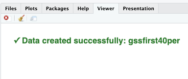
          • [[Highlighting and running]] this code will create a new data, gssfirst40per.
      • If the codes are correct, the [[viewer tab]] will provide confirmation:
        • 

[[Descriptive table]] #code for 40% non-random sampling¶

• [[Model code]]

  • 1	descr(gssfirst40per$variable_here, out = "v", show = "short")

• [[Working code]]

  • 1	descr(gssfirst40per$coninc, out = "v", show = "short")

    • Line 1: We put coninc here ➜ variable_here. Note that we use gssfirst40per instead of gss.
      • [[Find this working code in the R script file]].
        • [[Highlighting and running]] this code will generate the output below (which will appear in the [[viewer tab]] of RStudio).

[[Descriptive table]] #output for 40% non-random sampling¶

• Basic descriptive statistics

  • variable	variable label	n	NA.prc	mean	sd
    coninc	Respondents' family income	1415	11.23	53688.98	44151.37

[[Descriptive table]] #interpretation for 40% non-random sampling¶

• Non-random sampling descriptive table interpretation sample

  The overall respondents' family income mean among GSS respondents is $47,738, while the family income mean with a 40% non-random sample is $53,688.

  In this case since the mean family incomes differ by more than $3,000, we can conclude that these mean family incomes are substantially different.

  • Is a non-random sample preferable method for obtaining generalizable results?

    • It is not preferable; samples that are non-random cannot represent a whole population because all the individuals in the population do not receive equal chances of being selected.
    • Substantially different results were obtained about the family income means because non-random samples are not capable of representing the population as a whole.

• Non-random sampling descriptive table interpretation template

  The overall [[variable label]] mean among GSS respondents is mean, while the variable label mean with a sampling method name is mean.

  In this case since the mean variable label differ by more than threshold, we can conclude that these mean variable label are substantially different.

  OR

  In this case since the variable label do not differ by more than threshold, we can conclude that these mean variable label are not substantially different.

[[Simple random sampling]]¶

• In simple random sampling, each individual has an equal probability of selection, without considering any other criteria. If the sample frame is know, we can:
  • List all individual and number them consecutively, and
  • Use random numbers to select individuals.

• There are five steps in selecting a simple random sample:

  1. Obtain a complete list of individuals.
  2. Give each individual a unique number starting at one
  3. Decide on the required sample size.
  4. Select numbers for the sample size from a table of random numbers.
  5. Select the individuals that correspond to the randomly chosen numbers.

• Number	Name	Number	Name	Number	Name
  1	Adams, H.	18	Iulianotti, G.	35	Quinn, J.
  2	Anderson, J.	19	Ivono, V.	36	Reddan, R.
  3	Baker, E.	20	Jabornik, T.	37	Risteski, B.
  4	Bradsley, W.	21	Jacobs, B.	38	Sawers, R.
  5	Bradley, P.	22	Kennedy, G.	39	Saunders, M.
  6	Carra, A.	23	Kassem, S.	40	Tarrant, A.
  7	Cidoni, G.	24	Ladd, F.	41	Thomas, G.
  8	Daperis, D.	25	Lamb, A.	42	Uttay, E.
  9	Devlin, B.	26	Mand, R.	43	Usher, V.
  10	Eastside, R.	27	McIlraith, W.	44	Varley, E.
  11	Einhorn, B.	28	Natoli, P.	45	Van Rooy, P.
  12	Falconer, T.	29	Newman, L.	46	Walters, J.
  13	Felton, B.	30	Ooj, W.	47	West, W.
  14	Garratt, S.	31	Oppenheim, F.	48	Yates, R.
  15	Gelder, H.	32	Peters, P.	49	Wyatt, R.
  16	Hamilton, I.	33	Palmer, T.	50	Zappulla, T.
  17	Hartnell, W.	34	Quick, B.

GSS example 2: 30% simple random sampling¶

• We'll choose 30% of the GSS respondents in a random way.
  • First, create a new dataset for the 30% of the GSS respondents that will be chosen randomly.

[[Data creation]] #code for 30% simple random sampling¶

• [[Working code]]

  • 1	gssrandom30per <- gss[sample(nrow(gss), round(0.30 * nrow(gss))), ]

    • Line 1: gssrandom30per is the name of the new dataset.
      • This will appear under gss in Data Environment;
      • 0.30 is 30%.
        • [[Find this working code in the R script file]].
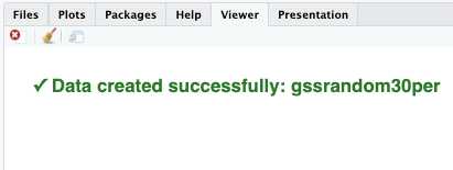
          • [[Highlighting and running]] this code will create a new data, gssrandom30per.
      • If the codes are correct, the [[viewer tab]] will provide confirmation:
        • 

[[Descriptive table]] #code for 30% simple random sampling¶

• [[Model code]]

  • 1	descr(gssrandom30per$variable_here, out = "v", show = "short")

• [[Working code]]

  • 1	descr(gssrandom30per$coninc, out = "v", show = "short")

    • Line 1: We put coninc here ➜ variable_here. Note that we use gssrandom30per instead of gss.
      • [[Find this working code in the R script file]].
        • [[Highlighting and running]] this code will generate the output below (which will appear in the [[viewer tab]] of RStudio).

[[Descriptive table]] #output for 30% simple random sampling¶

• Basic descriptive statistics

  • variable	variable label	n	NA.prc	mean	sd
    coninc	Respondents' family income	1067	10.79	46641.97	40957.59

[[Descriptive table]] #interpretation for 30% simple random sampling¶

• The overall respondents' family income mean among GSS respondents is 47,738 dollars, and we found 46,641 dollars. This is close! However, when you run those codes, you found a different mean. Also...

  • Here's the issue

    • If you run the data creation code and the descriptive table code again, you will find different results.
      • It's because every single time the data creation code is run, RStudio chooses different 30% of the GSS respondents.
        • There's an inconsistency issue.

  • 30% simple random sampling descriptive table interpretation sample

    The overall family income mean among GSS respondents is $47,738, while the family income mean with a 30% simple random sample is $46,641.

    In this case since the mean family incomes differ by more than $3,000, we can conclude that these mean family incomes are substantially different. In this case since the mean family incomes do not differ by more than $3,000, we can conclude that these mean family incomes are not substantially different.

    • Is a 30% simple random sample preferable to a non-random sample?

      • It is preferable; 30% simple random sampling is better than and superior to non-random sampling as there is a random selection. However, with each time the code is run, there is a different result.
      • Even though this method is better than non-random sampling, there is still inconsistency, as a different 30% of the data is selected each time.

  • 30% simple random sampling descriptive table interpretation template

    The overall [[variable label]] mean among GSS respondents is [mean], while the variable label mean with a sampling method is [mean].

    In this case since the mean variable label differ by more than [threshold], we can conclude that these mean variable label are substantially different.

    OR

    In this case since the variable label do not differ by more than [threshold], we can conclude that these variable label are not substantially different.

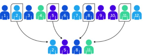
[[Systematic random sampling]]¶

• Systematic random sampling is same as simple random sampling, except: Choosing individuals from a random starting point, and choosing every nth individual (e.g., every 3rd individual).
  • 

• There are five steps in selecting a systematic random sample:

  1. Determine population size (e.g. 100).
  2. Determine sample size required (e.g. 20).
  3. Calculate sampling fraction (population / sample) (100/20=5)
  4. Select random staring point within first 5 cases (e.g. 3).
  5. Select every 5th case.

• Number	Number	Number	Number	Number
  01	21	41	61	81
  02	22	42	62	82
  03	23	43	63	83
  04	24	44	64	84
  05	25	45	65	85
  06	26	46	66	86
  07	27	47	67	87
  08	28	48	68	88
  09	29	49	69	89
  10	30	50	70	90
  11	31	51	71	91
  12	32	52	72	92
  13	33	53	73	93
  14	34	54	74	94
  15	35	55	75	95
  16	36	56	76	96
  17	37	57	77	97
  18	38	58	78	98
  19	39	59	79	99
  20	40	60	80	100

GSS example: 20% Systematic random sampling¶

• We'll choose 20% of the GSS respondents in a random way, with assigning the starting point and the choosing interval.
  • First, create a new dataset for the 20% of the GSS respondents that will be chosen randomly and systematically.

[[Data creation]] #code for 20% Systematic random sampling¶

• [[Working code]]

  • 1	gss20persystematic <- gss[seq(4, nrow(gss), 5), ]

    • Line 1: gss20persystematic is the name of the new dataset.
      • This will appear under gss in Data Environment;
      • 4 is the starting point, so the sample begins with the 4th respondent;
      • 5 means every fifth respondent is selected after that. Because 1 out of every 5 cases is chosen, the sample includes about 20% of the dataset.
        • [[Find this working code in the R script file]].
          • [[Highlighting and running]] this code will create a new data, gss20persystematic.
      • If the codes are correct, the [[viewer tab]] will provide confirmation:
        • 

[[Descriptive table]] #output for 20% Systematic random sampling¶

• Basic descriptive statistics

  • variable	variable label	n	NA.prc	mean	sd
    coninc	Respondents' family income	706	11.42	47838.77	41591.10

[[Descriptive table]] #interpretation for 20% Systematic random sampling¶

• The overall respondents' family income mean among GSS respondents is 47,738 dollars, and we found 47,838 dollars. This is extremely close!

  • 20% systematic random sampling descriptive table interpretation sample

    The overall family income mean among GSS respondents is $47,738, while the family income mean with a 20% systematic random sample is $47.838.

    In this case since the mean family incomes do not differ by more than $3,000, we can conclude that these mean family incomes are not substantially different.

    • Is a 20% systematic random sample preferable to a 30% simple random sample?

      • It is preferable; systematic random sampling method provides consistency, and even if there were fewer people used in this sampling, this is better than 30% simple random sampling.

      • Sampling is less about the size of the sample and more about the representativeness of the sample selected.

  • 20% systematic random sampling descriptive table interpretation template

    The overall [[variable label]] mean among GSS respondents is [mean], while the [[variable label]] mean with a sampling method is [mean].

    In this case since the mean [[variable label]] differ by more than [threshold], we can conclude that these mean [[variable label]] are substantially different.

    OR

    In this case since the [[variable label]] do not differ by more than [threshold], we can conclude that these [[variable label]] are not substantially different.