03. Descriptive statistics⚓︎

Module items⚓︎

R Script file⚓︎

Copy the code below ➜ Paste into [[RStudio console]] ➜ Hit Enter

source(url("https://raw.githubusercontent.com/ttezcann/ssric-reg/refs/heads/main/regression/docs/assets/r-scripts/0_packages_data.R")); 
download.file("https://raw.githubusercontent.com/ttezcann/ssric-reg/refs/heads/main/regression/docs/assets/r-scripts/03-descriptive.r", "03-descriptive.r"); 
file.edit("03-descriptive.r")

Lab assignment⚓︎

Descriptive statistics

Sample lab assignment⚓︎

Sample: Descriptive statistics

Learning outcomes⚓︎

1. Learn the differences between categorical (binary, nominal, ordinal) and continuous variables
2. Learn how to run and interpret frequency tables
3. Learn how to run and interpret descriptive tables
4. Learn how to create bar graph and histogram graph
5. Learn model codes and working codes structure

Suggested reading⚓︎

What is [[variable]]?⚓︎

• A variable is any characteristics, number, or quantity that can be measured or counted.
  • It represents any piece of information we know about our subjects (e.g., individuals).

[[Content of the variable]]⚓︎

• Based on the content of the variable, what it asks, there are two types of variables:
  • (1) [[Demographic variables]]
    • Questions about respondents’ demographics are called demographic variables or control variables, such as education, age, gender, income, race/ethnicity.
  • (2) [[Contextual variables]]
    • Questions about respondents’ attitudes, beliefs, or behaviors, are called contextual variables, such as happiness, environmental attitudes, friendship networks, social trust.

[[Types of the variable]]⚓︎

• Based on the way it is asked and the nature of it, there are two main types of the variables, which are important for data analysis.
  • They could be categorical or continuous.

[[Categorical]] variables⚓︎

• Categorical variables take on values that are labels.
  • Variables are categorical when respondents are provided responses to choose from.

• Values are NOT real numbers.

  • In the response set below, (3) no is not triple of (1) yes.

    Categorical variable

    Do you like coffee?
    (1) yes
    (2) not much
    (3) no

• Depending on the response categories, such as (1) yes, (2) not much, (3) no, there are three different categorical variables, described as below.

[[Binary]] variables⚓︎

• Binary variables include two responses.

  • Examples include true-or-false and yes-or-no questions.

    Binary variable

    Are you satisfied with your current job?
    (1) yes
    (2) no

[[Nominal]] variables⚓︎

• Nominal variables have more than two responses to choose from.

  • One more response category makes a binary variable a nominal.

    Nominal variable

    What is your job status?
    (1) working full time
    (2) working part time
    (3) unemployed

[[Ordinal]] variables⚓︎

• Ordinal variables have responses that can be put in a logical and hierarchical order.
  • Values are rank ordered.
    • For example, below there's a logical order from (1) not satisfied at allto (5)very satisfied
  • The differences between the responses are unknown or inconsistent.
    • For example, (2) not satisfied is not double of (1) not satisfied at all.

  • We do not treat the values of categorical variables as real numbers.

    Ordinal variable

    How satisfied are with your current job?
    (1) not satisfied at all
    (2) not satisfied
    (3) more or less
    (4) satisfied
    (5) very satisfied

Continuous variables⚓︎

• [[Continuous]] variable values represent real numbers.
  • When respondents are NOT provided options to choose from.

  • Here, the age of 20 is double of the age of 40, so it is continuous.

    Continuous variables

    What is your age?
    20, 40, 48, 80

    What is your income?
    $10,000, $30,000, $48,500

    How many years of schooling did you complete?
    10, 15, 17, 20

Determining variable type exercise⚓︎

• Determining the type of variable is important because different analysis techniques are used depending on the variable type.
  • Some questions from different surveys will be shown.

  • We will determine if they are;

    • Categorical (If so, binary, nominal, or ordinal)
    • Continuous
    1. Youth Participatory Politics Survey Project

    "I am interested in political issues. Do you..."

    1	2	3	4
    Strongly disagree	Disagree	Agree	Strongly agree

    Show the answer

    Categorical (Ordinal)

    2. American Health Values Survey

    "During the last 5 years do you think your health in general has gotten better, gotten worse or stayed about the same?"

    1	2	3
    Better	Worse	Stayed about the same

    Show the answer

    Categorical (Ordinal)

    3. European Social Survey

    "And at what age, approximately, would you say men reach old age?"

    Type in age ...

    Show the answer

    Continuous

    4. Latino National Survey

    "Now I want to ask you about a particular child. Think about your child who had the most recent birthday and was enrolled in school last year. For the following questions please focus on this child."

    Is this child enrolled in public or private school?

    Value	Label
    1	Yes
    2	No

    Show the answer

    Categorical (Binary)

    5. National Surveys on Energy and the Environment

    "How likely is it that weather in the US is influenced by global warming?"

    1	2	3	4
    Very likely	Somewhat likely	Not likely	Not likely at all

    Show the answer

    Categorical (Ordinal)

    6. Latino Second Generation Study

    "What is the highest level of school your father has completed?"

    Value	Label
    1	No formal education
    2	1st, 2nd, 3rd, or 4th grade
    3	5th or 6th grade
    4	7th or 8th grade
    5	9th grade
    6	10th grade
    7	11th grade
    8	12th grade NO DIPLOMA
    9	HIGH SCHOOL GRADUATE - high school DIPLOMA or the equivalent (GED)
    10	Some college, no degree
    11	Associate degree
    12	Bachelor's degree
    13	Master's degree
    14	Professional or Doctorate degree

    Show the answer

    Categorical (Ordinal)

    7. National Survey on Drug Use and Health

    "About how many days out of 365 in the past 12 months were you totally unable to go to school or work or carry out your normal activities"

    Number of days ...

    Show the answer

    Continuous

    8. New Family Structures Study

    "Thinking about your main job (for pay), which of the following sectors best describes your job?"

    1	2	3	4	5
    Private sector	Federal government	State or Local government	Non-profit sector	Self-employed

    Show the answer

    Categorical (Nominal)

    9. Police-Public Contact Survey

    "In the past 12 months, have you been involved in a traffic accident in which the police came to the scene?"

    1	2
    Yes	No

    Show the answer

    Categorical (Binary)

    10. Well-Being and Basic Needs Survey, United States

    "The following questions ask about you and your household. Are you now..."

    1	2	3	4	5
    Married	Widowed	Divorced	Separated	Never married

    Show the answer

    Categorical (Nominal)

[[Summary statistics]]⚓︎

• Summary statistics is used to obtain quick summaries of variables.
  • For [[categorical]] variables, we use:
    • [[Frequency table]]
    • [[Bar graph]]
  • For [[continuous]] variables, we use:
    • [[Descriptive table]]
    • [[Histogram graph]]

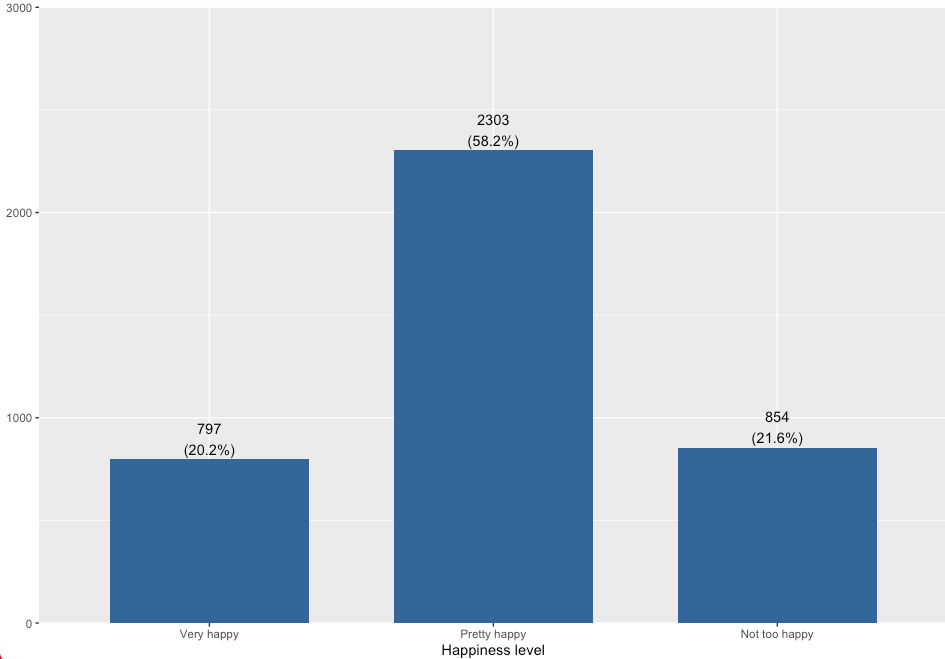
[[Frequency table]]⚓︎

• Frequency table is used to create a table showing the count and percentage for a single [[categorical]] variable.
  • The “Frequencies” (frq) code counts up how many times a response of a variable appears and calculates the percentage.
• We will create a frequency table for the finalter variable, then interpret it.

Find the variable in Variables in GSS page⚓︎

1. We want to make sure that finalter is a categorical variable. We check this information in the Variables in GSS page.

2. Search   Ctrl  /  Cmd+F  for the variable name, finalter. We see that this is a nominal, so a categorical variable.

   Variable name	Variable label	Variable type	Question wording and response categories
   finalter From: Variables in GSS	Perceived change in financial situation	Nominal	During the last few years, has your financial situation been getting better, worse, or has it stayed the same? (1: Better; 2: Worse; 3: Stayed same)

[[Frequency table]] #code⚓︎

• Model code

  1	frq(gss$variable_here, out = "v")

• Working code

  1	frq(gss$finalter, out = "v")

  • Line 1: We put finalter here ➜ variable_here. [[Highlighting and running]] this code will generate the output below (which will appear in the viewer part of RStudio).

[[Frequency table]] #output⚓︎

Perceived change in financial situation

• The next step will show interpretation.

  Use (valid.prc) in interpretations

  We always interpret the valid percentage column (valid.prc) as it excludes the missing data (NA), showing 30 respondents who did not respond to this question.

[[Frequency table]] #interpretation⚓︎

• After the [[variable label]], we add the word of "variable" in your interpretation:
  • "The Perceived change in financial situation variable shows that..."
• Depending on the variable, we need to tweak some parts of the interpretation.
  • For example, "15.4% of the respondents are/have/feel/think/said/reported" etc.
• We interpret the valid percentage column (valid.prc).

[[Bar graph]]⚓︎

• A bar graph is a visual representation of frequency table.
  • It provides the same information as [[frequency table]]. The interpretation is same as frequency table interpretation.
• We will create a bar graph for the satjob variable, then interpret it.

Find the variable in Variables in GSS page⚓︎

1. We want to make sure that satjob is a categorical variable. We check this information in the Variables in GSS page.

2. Search   Ctrl  /  Cmd+F  for the variable name, satjob. We see that this is a nominal, so a categorical variable.

   Variable name	Variable label	Variable type	Question wording and response categories
   satjob From: Variables in GSS	Level of work satisfaction	Ordinal	On the whole, how satisfied are you with the work you do? (1: Very satisfied; 2: Moderately satisfied; 3: A little dissatisfied; 4: Very dissatisfied)

[[Bar graph]] #code⚓︎

• Model code

  1 2 3

  plot_frq(gss$variable_here, type = "bar", geom.colors = "#336699")

• Working code

  1 2 3

  plot_frq(gss$satjob, type = "bar", geom.colors = "#336699")

  • Line 1: We put satjob here ➜ variable_here. [[Highlighting and running]] this code will generate the output below (which will appear in the plots part of RStudio).
  • Line 2: Instead of bar, we can use other arguments, such as density, box or line.

  • Line 3: We can change the bar color here. Replace the hex color code ➜ "#336699"

    Finding colors

    Browse and copy hex color codes at https://coolors.co/palettes/trending

[[Bar graph]] #output⚓︎

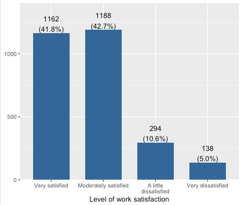
[[Bar graph]] #interpretation⚓︎

• After the [variable label], we add the word of "variable" in your interpretation:
  • "The level of work satisfaction variable shows that..."
• Depending on the variable, we need to tweak some parts of the interpretation.
  • For example, "15.4% of the respondents are/have/feel/think/said/reported" etc.
• Bar graphs already show the valid percentage (valid.prc).

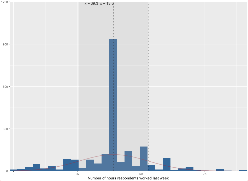
[[Descriptive table]]⚓︎

• Descriptive table is used to create a table showing the mean and standard deviation for a single [[continuous]] variable.

  • The “Descriptives” (descr) code is used to determine:
    • [[Mean]]:
      • The arithmetic average of a distribution, calculated by summing all observed values and dividing by the number of observations.
    • [[Standard deviation]]:
      • A measure of dispersion that quantifies the average distance of individual observations from the mean. A smaller standard deviation indicates that values are concentrated near the mean, while a larger standard deviation reflects greater variability across observations.

• We will create a descriptive table for the educ variable, then interpret it.

Find the variable in Variables in GSS page⚓︎

1. We want to make sure that educ is a continuous variable. We check this information in the Variables in GSS page.

2. Search   Ctrl  /  Cmd+F  for the variable name, educ. We see that this is a continuous variable.

   Variable name	Variable label	Variable type	Question wording and response categories
   educ From: Variables in GSS	Respondents' education in years	Continuous	What is the highest year of school you completed? (Min: 0, Max: 20)

[[Descriptive table]] #code⚓︎

• Model code

  1	descr(gss$variable_here, out = "v", show = "short")

• Working code

  1	descr(gss$educ, out = "v", show = "short")

  • Line 1: We put educ here ➜ variable_here.
    • [[Highlighting and running]] this code will generate the output below (which will appear in the viewer part of RStudio).

[[Descriptive table]] #output⚓︎

Basic descriptive statistics

[[Descriptive table]] #interpretation⚓︎

• After the [variable label], we add the word of "variable" in your interpretation:
  • "The respondents' education in years variable shows that..."
• Depending on the variable, we need to tweak some parts of the interpretation.
  • For example, "the average years of education is...", "the average weeks of working is..." etc.
• We use the mean (Mean column) and standard deviation (SD column) in our interpretation.

[[Histogram graph]]⚓︎

• Histogram graph is used to create a figure showing the mean and standard deviation for a single [[continuous]] variable. It provides the same information as descriptive table.
• We will create a histogram graph for the age variable, then interpret it.

Find the variable in Variables in GSS page⚓︎

1. We want to make sure that age is a continuous variable. We check this information in the Variables in GSS page.

2. Search   Ctrl  /  Cmd+F  for the variable name, age. We see that this is a continuous variable.

   Variable name	Variable label	Variable type	Question wording and response categories
   age From: Variables in GSS	Respondents' age	Continuous	What is your age? (Min: 18, Max: 89)

[[Histogram graph]] #code⚓︎

• Model code

  1 2 3

  plot_frq(gss$variable_here, type = "hist", normal.curve = T, show.mean = T, show.sd = T, geom.colors = "#336699", normal.curve.color = "#9b2226")

• Working code

  1 2 3

  plot_frq(gss$age, type = "hist", normal.curve = T, show.mean = T, show.sd = T, geom.colors = "#336699", normal.curve.color = "#9b2226")

  • Line 1: We put age here ➜ variable_here. [[Highlighting and running]] this code will generate the output below (which will appear in the plots part of RStudio).

  • Line 2: We can change the bar and curve color here separately. Replace the hex color code for bar ➜ "#336699". Replace the hex color code for curve ➜ "#9b2226"

    Finding colors

    Browse and copy hex color codes at https://coolors.co/palettes/trending

[[Histogram graph]] #output⚓︎

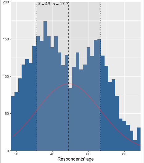
[[Histogram graph]] #interpretation⚓︎

• After the [variable label], we add the word of "variable" in your interpretation:
  • "The respondents' age variable shows that..."
• Depending on the variable, we need to tweak some parts of the interpretation.
  • For example, "the average age of the respondents is...", "the average weeks of working is..." etc.
• We use the mean and standard deviation in our interpretation.
  • The mean is indicated by x̄, the standard deviation is indicated by s (at the very top of the histogram graph)